Basic analysis of 10X example Visium dataset

Introduction

In this introductory notebook for VoyagerPy, we demonstrate basic exploratory data analysis (EDA) of spatial transcriptomics data. Basic knowledge of Python is assumed.

This notebook showcases the packages with a Visium spatial gene expression system dataset, downloaded from the 10X website, in the Space Ranger output format. The technology was chosen due to its popularity, and therefore the availability of numerous publicly available datasets for analysis (Moses and Pachter 2022).

VoyagerPy was developed with the goal of facilitating the use of geospatial methods in spatial genomics. However, this notebook is introductory to the package and is restricted to non-spatial scRNA-seq EDA with the Visium dataset.

Note: This notebook has an accompanying vignette in R, so we try to match the results as well as we can.

Note: Before running this notebook, make sure you have Scanpy, igraph, and leidenalg installed. These packages can be installed via pip install "scanpy[leiden]".

We start by loading the basic packages

import numpy as np
import geopandas as gpd
import pandas as pd

import scanpy as sc
import voyagerpy as vp

from matplotlib import pyplot as plt

# We set the dpi to get clearer figures
plt.rcParams['figure.dpi'] = 120  # The default is 100

# Turn on matplotlib interactive mode so we don't need to explicitly call plt.show()
plt.ion()

<contextlib.ExitStack at 0x7f697c3025e0>

Downloading the data

We download the raw count data from the 10X website. These are two gzipped tar archives containing the unfiltered gene count matrix and the spatial information. Thus, we unzip the files.

import requests
import pathlib
import json

outs_dir = pathlib.Path('data/visium_10x/outs')
outs_dir.mkdir(parents=True, exist_ok=True)
root_dir = (outs_dir / '..').resolve()

# Download the gene count matrix
tar_path_ob = root_dir / 'visium_ob.tar.gz'
url_reads = "https://cf.10xgenomics.com/samples/spatial-exp/2.0.0/Visium_Mouse_Olfactory_Bulb/Visium_Mouse_Olfactory_Bulb_raw_feature_bc_matrix.tar.gz"
if not tar_path_ob.exists():
    res = requests.get(url_reads)
    with tar_path_ob.open('wb') as f:
        f.write(res.content)

# Download the spatial information
tar_path_sp =  root_dir / 'visium_ob_spatial.tar.gz'
url_spatial = "https://cf.10xgenomics.com/samples/spatial-exp/2.0.0/Visium_Mouse_Olfactory_Bulb/Visium_Mouse_Olfactory_Bulb_spatial.tar.gz"
if not tar_path_sp.exists():
    res = requests.get(url_spatial)
    with tar_path_sp.open('wb') as f:
        f.write(res.content)

# Decompress the downloaded files
!tar -xvf $tar_path_ob -C $outs_dir
!tar -xvf $tar_path_sp -C $outs_dir

raw_feature_bc_matrix/
raw_feature_bc_matrix/features.tsv.gz
raw_feature_bc_matrix/barcodes.tsv.gz
raw_feature_bc_matrix/matrix.mtx.gz
spatial/
spatial/spatial_enrichment.csv
spatial/tissue_lowres_image.png
spatial/tissue_positions.csv
spatial/detected_tissue_image.jpg
spatial/aligned_fiducials.jpg
spatial/scalefactors_json.json
spatial/tissue_hires_image.png

This is what the layout of the outs directory looks like. The outputs in the spatial directory is explained here on the 10X website.

def print_dir_content(p, d=0):
    print(' '*(d*2) + p.name, end='/\n' if p.is_dir() else '\n')
    if p.is_dir():
        for sub in sorted(p.iterdir()):
            print_dir_content(sub, d+1)

has_tree = !command -v tree
if has_tree:
    !tree $outs_dir
else:
    print_dir_content(outs_dir)

outs/
  raw_feature_bc_matrix/
    barcodes.tsv.gz
    features.tsv.gz
    matrix.mtx.gz
  spatial/
    aligned_fiducials.jpg
    detected_tissue_image.jpg
    scalefactors_json.json
    spatial_enrichment.csv
    tissue_hires_image.png
    tissue_lowres_image.png
    tissue_positions.csv

The tissue_hires_image.png file is a relatively high resolution image of the tissue, but not full resolution. The tissue_lowres_image.png file is a low resolution image of the tissue, suitable for quick plotting.

im = plt.imread(outs_dir/'spatial' / 'tissue_hires_image.png')
_ = plt.imshow(im, origin='lower')

The array of dots surrounding the tissue is the fiducials. These are used for aligning the image to the positions of the Visium spots, so gene expression can be matched to spatial locations. The alignment of the fiducials are shown in aligned_fiducials.jpg. Space Ranger can automatically detect which spots are in tissue. These spots are highlighted in detected_tissue_image.jpg and have in_tissue == 1 in tissue_positions.csv.

The scale_factors_json.json describes how we go from full-res coordinates to the lower resolution coordinates. It also contains the sizes of the spots and fiducials.

spot_diameter_fullres is the diameter of each Visium spot in the full resolution pixel space. The scalars tissue_hires_scalef and tisse_lowres_scalef are the ratios of the hires and lowres images to the fullres image. fiducial_diameter_fullres is the diameter of each fiducial in full resolution.

json.load((outs_dir / 'spatial' / 'scalefactors_json.json').open())

{'tissue_hires_scalef': 0.2,
 'tissue_lowres_scalef': 0.06,
 'fiducial_diameter_fullres': 118.91545,
 'spot_diameter_fullres': 73.61433}

The file tissue_positions.csv contains information for the Visium spots in the image; * barcode * in_tissue: whether the barcode is covered by tissue (1) or not (0), as detected by Space Ranger, or manually annotated in the Loupe browser. * array_row / array_col: The grid position of the spot on the Visium slide. * pxl_row_in_fullres / pxl_col_in_fullres: The pixel position of the spots in the full resolution image.

pd.read_csv(outs_dir / 'spatial' / 'tissue_positions.csv').head()

	barcode	in_tissue	array_row	array_col	pxl_row_in_fullres	pxl_col_in_fullres
0	ACGCCTGACACGCGCT-1	0	0	0	8668	1102
1	TACCGATCCAACACTT-1	0	1	1	8611	1200
2	ATTAAAGCGGACGAGC-1	0	0	2	8554	1102
3	GATAAGGGACGATTAG-1	0	1	3	8498	1200
4	GTGCAAATCACCAATA-1	0	0	4	8441	1102

The file spatial_enrichment.csv contains some information for the genes, e.g. Moran’s I and its p-value.

pd.read_csv(outs_dir / 'spatial' / 'spatial_enrichment.csv').head()

	Feature ID	Feature Name	Feature Type	I	P value	Adjusted p value	Feature Counts in Spots Under Tissue	Median Normalized Average Counts	Barcodes Detected per Feature
0	ENSMUSG00000001023	S100a5	Gene Expression	0.770905	0.0	0.0	9019	15.848669	1021
1	ENSMUSG00000019874	Fabp7	Gene Expression	0.698735	0.0	0.0	13462	20.679932	1170
2	ENSMUSG00000002985	Apoe	Gene Expression	0.694521	0.0	0.0	67509	76.635169	1184
3	ENSMUSG00000025739	Gng13	Gene Expression	0.658575	0.0	0.0	5260	8.803694	1050
4	ENSMUSG00000090223	Pcp4	Gene Expression	0.631703	0.0	0.0	45118	25.811125	1133

Here we read the Space Ranger output as an AnnData object. Since we have the raw counts, we set raw = True. The count matrix is in .mtx format, and we want to load the lowres image.

adata = vp.read_10x_visium(
    outs_dir,
    datatype = 'mtx',
    raw = True,
    prefix = None,
    symbol_as_index=False,
    dtype=np.float64,
    res='lowres'
)

We can use VoyagerPy to display the image stored in the adata object.

_ = vp.plt.imshow(adata)

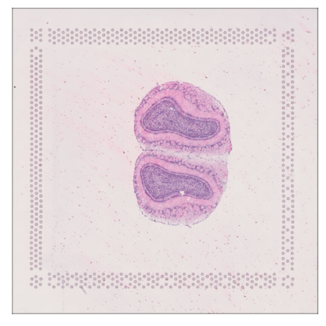
The images and coordinates of the Visium spots are aligned. However, according to the 10X website, a properly aligned slide image should have the hourglass in the top-left corner and the triangle on the bottom left. The rotation of the image does not affect any of the computations, but VoyagerPy offers a way to rotate/mirror the image and the spot coordinates. Here, we rotate and mirror the image to match the fiducials.

fig, axs = plt.subplots(2, 2, figsize=(10,10))

vp.plt.imshow(adata, ax=axs[0,0], title='Original')

vp.spatial.rotate_img90(adata, k=1, apply=False)
vp.plt.imshow(adata, tmp=True, ax=axs[0,1], title='Rotated 90° clockwise - not applied')

vp.spatial.mirror_img(adata, axis=1, apply=False)
vp.plt.imshow(adata, tmp=True, ax=axs[1, 0], title='Mirror rows - not applied')

vp.spatial.apply_transforms(adata)
_ = vp.plt.imshow(adata, ax=axs[1,1], title='Transformed image - changes applied')

Quality Control (QC)

We start off by computing some basic QC metrics for the dataset.

is_mt = adata.var['symbol'].str.contains('^mt-').values
vp.utils.add_per_cell_qcmetrics(adata, subsets={'mito': is_mt})

Now, we need a way to show display data with respect to their histological location. Since we are dealing with a 10X Visium dataset, we know how to access this information. Thus, we add the visium spots as the representative geometry of the barcodes.

visium_spots = vp.spatial.get_visium_spots(adata, with_radius=True)

# Set the geometry to the visium spots and assign the name "spot_poly"
_ = vp.spatial.set_geometry(adata, geom="spot_poly", values=visium_spots)

Since we have defined the barcode geometry, we can plot the QC metrics in tissue space.

qc_features = ["sum", "detected", "subsets_mito_percent"]
axs = vp.plt.plot_spatial_feature(
    adata,
    qc_features,
    image_kwargs=dict(),
    subplot_kwargs=dict(figsize=(8,8), dpi=100, layout='tight')
)

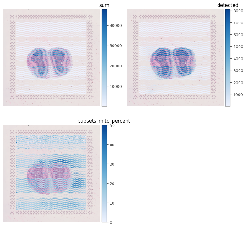
The percentage of mitochondrial counts (subsets_mito_percent) in spots outside tissue is higher near the tissue, especially on the left. See the figure above.

# set the `in_tissue` as a categorical variable.
adata.obs['in_tissue'] = adata.obs['in_tissue'].astype(bool).astype('category')

axs = vp.plt.plot_barcode_data(
    adata,
    y=qc_features,
    x='in_tissue',
    ncol=3,
    figsize=(8, 4),
    cmap='tab10',
)

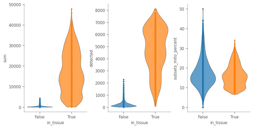
Here we can see see three peaks, apparently histologicaly relevant, but no obvious outliers.

_ = vp.plt.plot_barcode_data(
    adata,
    x='sum',
    y='subsets_mito_percent',
    color_by='in_tissue',
    cmap='tab10',
    contour_kwargs=dict(colors='blue', levels=9),
)

This is unlike scRNA-data. Spots not in tissue have a wide range of mitochondrial percentage. Spots in tissue fall into three clusters in the above plot, seemingly related to histological regions.

Now, we select only visium spots covered by the tissue. Due to the internals of AnnData, we must copy the sliced object and set the geometry of adata_tissue again.

adata_tissue = adata[adata.obs["in_tissue"]==True].copy()
vp.spatial.set_geometry(adata_tissue, "spot_poly")

AnnData object with n_obs × n_vars = 1185 × 32285
    obs: 'in_tissue', 'array_row', 'array_col', 'pxl_row_in_fullres', 'pxl_col_in_fullres', 'sum', 'detected', 'subsets_mito_sum', 'subsets_mito_detected', 'subsets_mito_percent'
    var: 'symbol', 'feature_types'
    uns: 'config', 'spatial', 'metadata'
    obsm: 'geometry'

ax = vp.plotting.plot_barcodes_bin2d(
    adata_tissue,
    x='sum',
    y='detected',
    bins=76,
    figsize=(10, 7)
)

In order to preserve the counts and the log-normalized counts, we save them as layers. This is because we will normalize adata_tissue.X before we perform PCA in this notebook.

# The original count data
adata_tissue.layers['counts'] = adata_tissue.X.copy()
# Log-normalize the adata.X matrix
vp.utils.log_norm_counts(adata_tissue, inplace=True)
adata_tissue.layers['logcounts'] = adata_tissue.X.copy()

Next, we select the top 2000 highly variable genes. We use the model_gene_var to model the variance of the gene expression, decomposing the perceived variance into biological variance and technological variance. The biological variance is what we are interested in.

gene_var = vp.utils.model_gene_var(adata_tissue.layers['logcounts'], gene_names=adata_tissue.var_names)
hvgs = vp.utils.get_top_hvgs(gene_var)

# Set the 'highly_variable' column for the genes
adata_tissue.var['highly_variable'] = False
adata_tissue.var.loc[hvgs, 'highly_variable'] = True

Dimension reduction and clustering

In the companion vignette, the data is scaled prior to computing the PCA. Thus, we follow suit.

# scale first, then perform pca

adata_tissue.X = vp.utils.scale(adata_tissue.X, center=True)
sc.tl.pca(adata_tissue, use_highly_variable=True, n_comps=30, random_state=1337)
adata_tissue.X = adata_tissue.layers['logcounts'].copy()

_ = vp.plt.elbow_plot(adata_tissue, ndims=30)

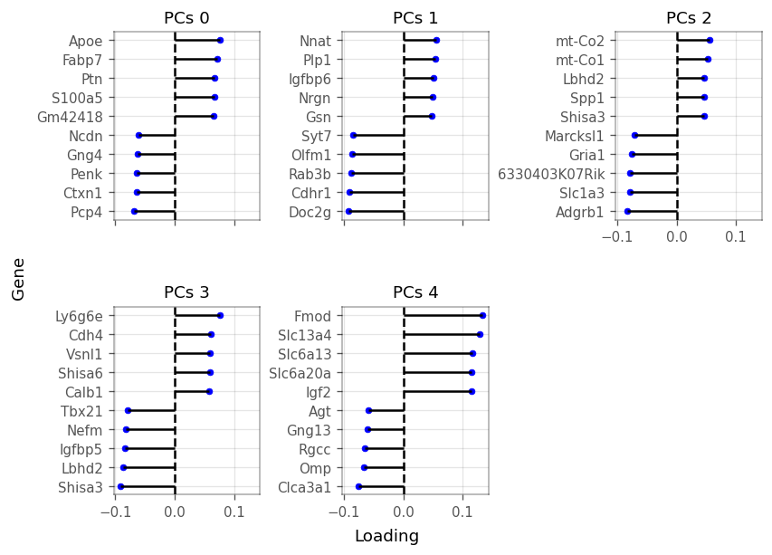
ax = vp.plt.plot_dim_loadings(
    adata_tissue,
    range(5),
    show_symbol=True,
    ncol=3,
    figsize=(7, 5),
)

Cluster the barcodes in PCA space. We adjusted the n_neighbors parameter to find similar clustering as in the R vignette.

from leidenalg import ModularityVertexPartition

sc.pp.neighbors(
    adata_tissue,
    n_pcs=3,
    use_rep='X_pca',
    method='gauss',
    n_neighbors=80
)
sc.tl.leiden(
    adata_tissue,
    random_state=29,
    resolution=None,
    key_added='cluster',
    partition_type=ModularityVertexPartition
)

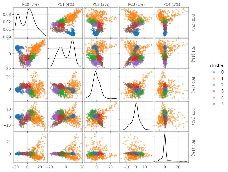
ax = vp.plt.plot_pca(
    adata_tissue,
    figsize=(7,7),
    ndim=5,
    color_by='cluster',
    cmap='tab10',
)

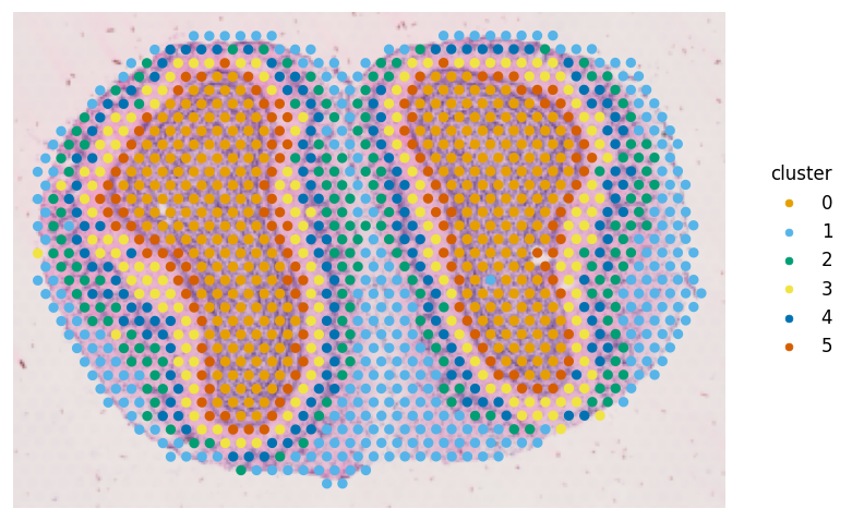
ax = vp.plt.plot_spatial_feature(
    adata_tissue,
    'cluster',
    barcode_geom='spot_poly',
    image_kwargs=dict(crop=True, pad=10),
)

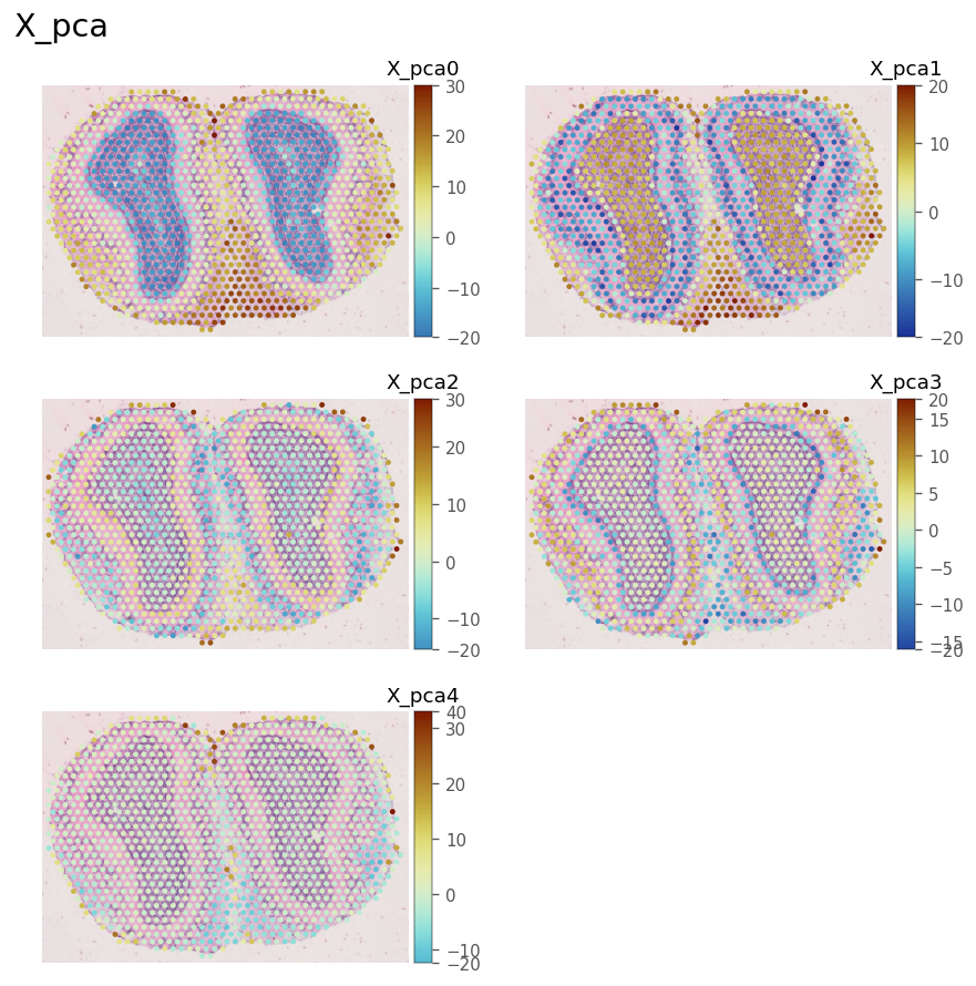
pl = vp.plt.spatial_reduced_dim(
    adata_tissue,
    "X_pca",
    ncomponents=5,
    ncol=2,
    divergent=True,
    figsize=(7,7),
    image_kwargs=dict(crop=True),
)

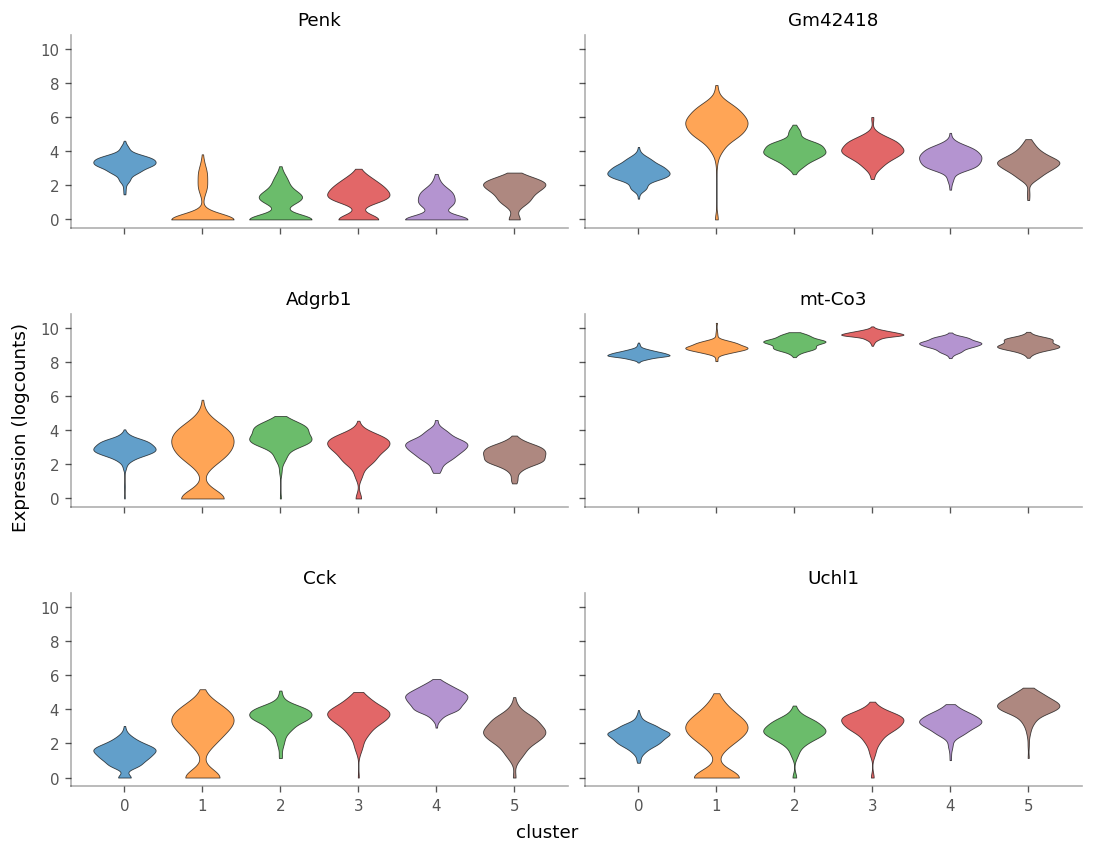
Significant markers for each cluster are obtained as follows. Note, that since the clustering is not identical between bluster and Scanpy, the marker genes will vary slightly.

markers = vp.utils.get_marker_genes(adata_tissue, False, cluster='cluster')
marker_genes = markers.iloc[0, :].tolist()

adata_tissue.var.loc[marker_genes, ['symbol']]

	symbol
ENSMUSG00000045573	Penk
ENSMUSG00000098178	Gm42418
ENSMUSG00000034730	Adgrb1
ENSMUSG00000064358	mt-Co3
ENSMUSG00000032532	Cck
ENSMUSG00000029223	Uchl1

_ = vp.plt.plot_expression(
    adata_tissue,
    marker_genes,
    groupby='cluster',
    show_symbol=True,
    layer='logcounts',
    cmap='tab10',
    figsize=(9,7),
    scatter_points=False
)

These genes show some interesting patterns in spatial context:

_ = vp.plt.plot_spatial_feature(
    adata_tissue,
    marker_genes,
    ncol = 2,
    layer='logcounts',
    subplot_kwargs=dict(
        figsize=(7,7),
        layout='constrained',
    ),
    image_kwargs=dict(crop=True)
)